Youtube's Homepage Recommendations

These are my notes on the popular Youtube RecSys paper, I decided to blog them both for my own future reference and if maybe somebody benefits from reading my thought process on these systems. This paper’s about “the most sophisticated industrial recommendation system in existence”. Let me first define my learning objectives for this paper, of what I expect to learn from it:

• Large scale ML system design (how to scale to a massive dataset of candidate items)
• Real time inference (how they have sub-millisecond latency on such a system)
• Any specific training requirements of a system this large.

The abstract says both candidate generation and ranking are done using a deep model, this should be interesting.

Appreciating Youtube’s Scale

Challenges

• The problem scale is so large most existing algorithms fail.
• A parallel to exploration exploitation:
  • Youtube has a lot of new videos and user preferences are constantly changing.
  • The recsys can’t be a one and done system.
• Noise:
  • There’s obviously a lot of external factors that make historical predictions difficult.
  • Sparisty in the user feature vectors (large number of items)
  • All feedback has to be implicit as user explicit feedback (like/dislike) is rare.
  • No proper arrangement of the ontology (labels are not hierarchical and not normalised)

Model Scale

• Model is Billion parameter scale.
• Model is trained using hundreds of billions of samples (infinite data glitch).
• Latency requirements are in the order of sub-millisecond.
• Probably related to the above, the last system is a logistic regression.
• It’s modified for watch time prediction instead of CTR.

Takeaway: My understanding is at training time you can do whatever deep-learning you want to do but the inference has to be done using linear systems. Nothing else will scale. Which is surprising given how everything is transformers now which are quadratic time.

Hidden layer depth is helpful in this situation? Probably to make the features more linearly separable. Probably they just have so much data so more depth is always good as long as they can train (didn’t have resnet50 at the time so no residual connections are used).

System Overview

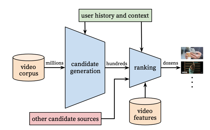
• Candidate generation neural net and ranking neural net
• Models user’s Youtube activity
• System1 is required to be high precision
  • This system is a coarse personalization where it gives hundreds of suggestions
  • A precision metric tracking means that if it recommends 100 items, we try to minimise the presence of any irrelevant items
• System2 is high recall
  • Recall means all relevant items should be present.
  • If it’s recall@10 then conceptually missing any relevant items penalizes the model.
  • If it’s precision@10 then it doesn’t matter that we miss relevant items.
  • Let’s say to optimise precision our model only recommends 3 items, whereas it has a budget of 10
  • This would give it 100% precision while we were ok with lower percision.
  • Users are not exactly sure what they’re looking for.
  • We can miss a click opportunity by trying to optimise for precision.

My opinion is that for a business it would come down to how costly it’s for them to be “wrong” about certain things. For example, Linkedin might want to only show highly relevant jobs and none at all if they don’t exist. If you think about it, sometimes they only show 3-4 jobs. They might therefore be optimising for high precision.

Youtube on the other hand doesn’t think twice before recommending Vlog spam crap and we just blame it on demographics of the country instead of losing trust in this system.

High precision on the ranking would therefore be useful when it’s critical to maintain the user’s trust in the system.

Finally, they talk about offline vs online metrics. The metrics they track online are:

• Click Through rate changes
• Watch time

This is obviously because the system is temporal and there is no perfect way to determine whether past behaviour is indicative of future behaviour.

Candidate generation at scale

It’s obvious to even the most casual observer that Youtube needs to recommend from a very large corpus. There are the below problems that I imagine they would have:

• New videos - when do you include these?
• As mentioned by the authors how do you incoroporate the temporal aspect
• How do you scale to the massive size of this corpus
• How do you reach sub-millisecond latency

The system they have described is their personalization candidate generation system, I imagine when it’s not available, to solve the cold start problem they have a different candidate generation method (they’ve mentioned secondary sources in the paper).

Another possible solution to the cold start problem can be computing item embeddings using an average of known properties such as averaging other uploads of the uploading user or prefernces of the users who have interacted with the video after it has had the first few initial views.

• The earlier system to do this was a matrix factorisation system trained with rank loss
• Which begs the question, why switch?
• The matrix factorisation technique was equivalent to a shallow network that only embeds user’s watch history (user preference vector)
• The new deep network is therefore a non-linear generalisation of it.
• Imagine it worked better?

This blog post I found via good old fashioned Googling is on the topic of WARP which is the ranking loss used to train the previous matrix factorisation based candidate generation model.

Excerpts that summarise the blog post above:

• Problem: Recommend item i to user u, f_u(i) will be the score of item i for user u
• For each (u, i) pair choose an item i’ that is ranked higher than i
• There’s a function that estimates the rank of each item.
• Use the rank estimates’ function to perform gradient updates.
• Amplified updates if the model deems (u, i) implausible
• rank(i, u) = sum(i’ such that i’ is ranked higher than i)
• precision@k is maximised when log(rank) is minimised (somebody proved this result)
• Rank as defined above is not continuous and therefore difficult to train a ML model with using gradients.
• log(rank) is differentiable and that is minimised instead.
• Derivation of the paper is nonsense (I agree)
• Overall it can be seen as the hinge loss applied to rank and we want its expected value
• calculating rank(i) requires calculating scores for all items
• That paper approximates it by checking how many negatives were drawn before we found a non-negative and approximates
• This is non-differentiable and therefore applied as weighting to the loss (the hinge loss between negative and positive)
• You then train it.

So anyway, that was the old matrix factorisation based approach and for anybody else looking for a refresher, recommended rabbit hole to go down. Fair warning there’s a bunch of other rabbit holes ahead for anybody rusty with RecSys like me.

Formulation as a classification problem

• Obviously when you do this, it becomes extreme classification with so many candidates
• Again there’s a temporal aspect to it, you’re predicting watch@time_t.
• They use a softmax formulation, each class score is u.v where u is the user vector and it’s dotted with item vector v_j.
• That class score is then fed through softmax normalisation.
• Since there’s two different input features for this softmax, those will need to be learned.
• An additional tidbit is u is an embedding for user history U and context C. It is not clearly defined what this C is.
• The embeddings are not continuous, the idea is just for them to be a dense compression of sparse feature vectors.
• So then v_j is likely just video ids and u is something to be learned using the deep network.
• Positive sample - user watches a video in full (probably would be around 80% or so to account for pre-roll skips etc)
• This is less sparse than likes/dislikes although it’s implicit.

How they trained for extreme multiclass efficiently

• Sample negative classes from a background distribution
• This is, as you’d need to train some sort of ranking here which will require triplets
• Since they sample these, the sampling is corrected for in the loss via importance weighting
• Minimise cross-entropy loss, set it up by taking positive class = video watched. Negative classes = sampled negatives from the corpus
• Sample several thousand negatives, this is still not the entire label space.
• Instead of sampling could’ve used hierarchical softmax
  • Hierarchical softmax: Reduce computational complexity to log_{- 2}(V).
  • Ruder has a good post on both this and importance sampling, these techniques were quite popular in 2016 and is therefore assumed knowledge for the paper.
  • This is, because this was in the pre sub-word tokenisation era and language modeling, for which it was developed used to have huge vocabularies.
  • Hierarchical softmax is BS because it doesn’t give a prediction time speedup, only one for training time.
  • It involves computing a tree structure over all words and connecting to the tree structure instead of the words themselves
  • The reason the authors give for discarding hierarchical softmax is the fact that the clusters of items are unrelated and therefore it makes the learning problem harder and the performance notably degrades.
• Importance weighting instead reduces the number of classes via sampling.
• Sampling is generally done when you know a distribution to find the expectation (Monte Carlo methods). If you knew the distribution however, there’s no learning task here.
• The general idea is that the denominator should be cheap to compute (which it won’t be if you did this with a million items)
• A proposal distribution needs to be used. I feel this idea is also what has now motivated speculative decoding.
• An option in language modeling is to use the distribution over unigrams, here it would be to do it based on the number of views.
• They however have not mentioned what proposal distribution they used.
• For infernce, they are using a NN search approach that looks quite similar to FAISS + embeddings (how?)
  • So this one was counterintuitive even for me to understand, but here’s how I think this works.
  • The general way this is done now is what’s called a “two tower approach” in which you train using a cosine similarity based pairwise ranking loss, two networks that create user and item embeddings.
  • If you’ve done NLP, you’d recognise the above as being the siamese architecture used in DPR, sentence transformers and other such similarity embedding techniques.
  • So the unintuitive part here, is to convince yourself that the video embedding they use and the user embeddings are in the same embedding space. With words it’s simpler to see, but you can convince yourself of the same by trying to think of what they’re treating as a video embedding in the nearest neighbor index - it’s the weights learned against each item in the last weight matrix (softmax l"layer") of the candidate generation network.
  • If a user vector is 1, i.e. the user does not have any preference the dot product output would be v_j itself.
  • So you can put those in an inverted index and then at runtime, query using the user vector’s embedding in that space for approximate nearest neighbors.
  • The user embedding itself can be thought of as the average of some “topics” and “creators” the user would be interested in at time t.

To drill down the last unintuitive part of this what helped me was this excellent blog post which I think is a bit inaccurate in that Youtube doesn’t do a two tower model in the “real” way it’s done today (I could be wrong but he doesn’t cite a post). There’s also this talk on Recommender Systems that I saw parts of and this Google developer link which in-passing and through that graphic really cconveys something beautiful.

Model specifics

Now, let’s try and make sense of the above extreme multiclass problem. They start by learning “video embeddings” simililar to learning word embeddings with a CBOW objective. The sequence they feed instead of sentences is a watch history sequence (so given 2n surrounding videos, need to predict the one in between.)

These are task specific embeddings, so they are mean pooled for input to the next layer (hidden layer of the deep network). Importantly, they are not goig to learning these separately by optimising logprob as in the case of CBOW, instead learn it jointly with the rest of the network.

For the first layer input, they combine it with other features:

• Embeddings of search queries are concatenated to video pool vector.
• The embeddings of search queries themselves are a pool of unigram + bigram embedding vectors.
• A bunch of real valued standard ML feature are engineered:
  • Demographics - device and location (categorical)
  • geneder
  • logged-in (yes/no)
  • age (normalised)
• Example age: This is a novel thing they came up with where in order to keep the recommendations fresh. When training, they wanted to encode that model’s making predictions at some temporal time T, so they encoded video age and set this to 0 for prediction to indicate prediction is at the end of the training window.
• Additionally, they want videos to go viral so this freshness is important. Otherwise they would just keep recycling videos. But they cannot lose relevance.
• Authors note on surrogate objectives - recommendation requires a surrogate like predicting ratings to carry over to video clicks. You cannot validate this surrogate on offline metrics.
• They generate examples for training from all over as they can’t have a recommender that only exploits pre-existing knowledge.
• Data balancing:- they didn’t have equality on labels but they used an equal number of samples from each user.
• Their surrogate objective is predicting the next watched video, which would be heavily affected by a recent search. You can’t simply throw results of that search query as the entire homepage.
• Solution: Represent search queries as a bag of words so classifier doesn’t learn their temporal ordering.
• Due to user behaviour patterns next watch prediction is a much better surrogate than simple “watch prediction”,basically CBOW is not good for them, they need a time-series style approach.
• They measure mAP at this stage, as position of all candidates is relevant and not just of the top k (that’s going to be in the ranking model).

Ranking Model

• The primary reason for the existence of this model is a lot of video features that you can’t use at scale can be incorporated.
• It is also used to combine candidates from different sources
• A weighted logistic regression is used to model expected watch time
• At prediction time, the vector is passed through the exponentiation function to generate odds
• They hand engineer a bunch of features since a lot of their features are quite sparse and can’t be directly fed to the model
• They touch on the importance of normsalisation of features
• The video embedding is shared between impressions/user watches etc
• Past impressions are incorporated as a feature so that the recommendations are not redundant (don’t keep recommending videos the user is never likely to watch)
• If the watch time for a video the user doesn’t click on is higher than the one they did click on, it’s a mis-prediction
• Weighted loss for the user is then calculated by dividing the above by total watch time
• An interesting feature engineering techinque is feeding powers and square roots which was found to be working well by nudging the model to learn those relationships
• Ranking by CTR promotes clickbait
• It is always better to model past user behaviour via some continuous feature like “how many videos of this creator has the user watched” over simply “has the user watched a video by this creator”
• We also use the scores of the candidate generators as a feature.
• Interesting, they chose to continue with a classification formulation for predicting a continuous value
• One reason can be normsalisation since videos are of different length?